6 Nov, 2018
Renderer Breakdown
The renderer in my demo uses a simple deferred pipeline that I will describe below. The goal of the project was to create a non-photorealistic renderer that would create images of a pleasing quality, not accurately replicate any visual properties found in the physical world. The project took many shortcuts, as it was completed entirely in my free time. As a result, there are many missed opportunities for better quality outcomes or more efficient approaches. However, these would have been more complicated and therefore more time consuming to program. I will do my best to call out these shortcomings as I move along. Additionally, I am self taught in the field of computer graphics, so I thank you for sifting through any misused terms you may encounter. I hope this document can be of some use either as educational or referential material for similar rendering projects, as I break down step by step the components of the renderer, from the beginning to the end of one frame.
As an overview, you can think of the pipeline as being broken down into three stages. First is the prep stage, where textures that will be used in the main render are created or filled out. This includes shadowmap generation, light shaft generation, ambient occlusion calculation, and filling the g-buffer's textures. Next is the main render which I consider a stage on it's own, and finally, the post processing effects which operate on HDR color textures, such as anti aliasing, bokeh blurring, and tonemapping. Now, I will dive into the details of each stage in sequence.
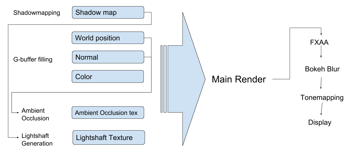
Renderer Overview, lines represent data dependency
Preparation Passes
The first step of the prep stage is a cascading shadowmap pass with three cascades. The view projection matrices for each cascade are generated from the view projection matrix that will be used in the main render by splitting the view frustum into pieces at chosen planes (parallel to the near and far plane), then calculating a sphere that encompasses the given frustum piece, and creating an orthographic view matrix that would capture the entirety of this sphere. As you can imagine, this coarse shadow camera creation matrix process leaves a lot of waste when compared to a hypothetical camera fit to the exact piece of the original frustum, but it makes for much simpler code. While other games/engines/apps use logarithmically progressing distances to split the view frustum, I chose my distances using the good old guess-and-check method.
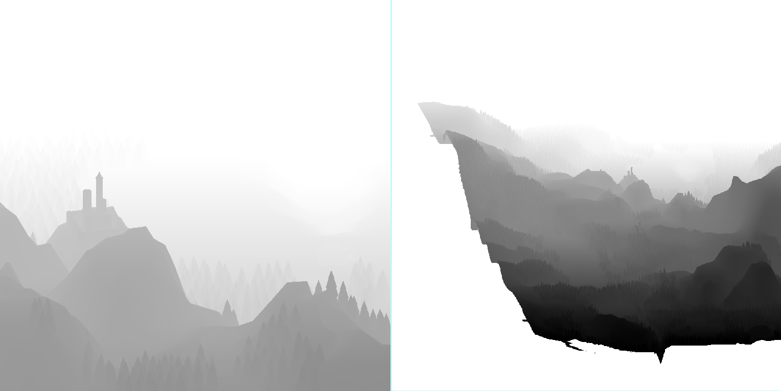
Two shadow cascades, from medium and far distances
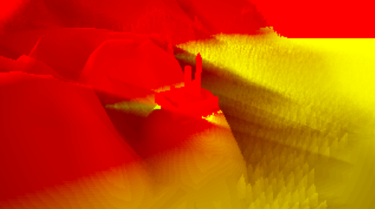
After the shadowmap pass comes the rendering of all scene geometry, filling in the g-buffer. The g-buffer consists of a normal texture, world position texture, color texture, and depth buffer. The first two are 4 channel 16-bit floating point textures and the color is an 8-bit 3 channel texture. It should be noted that one can squeeze similar precision out of an 8-bit floating point normal texture by applying a corrective formula that masks the gaps in accuracy caused by the lower bit count.
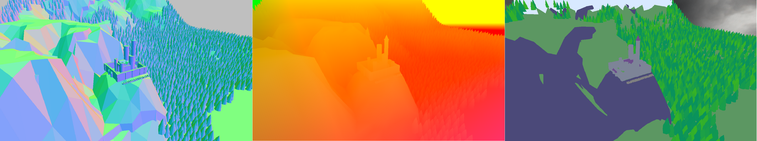
G Buffer: Normal, World Position, and Color Textures
The next pass calculates ambient occlusion in screenspace. The pass implements a standard algorithm which samples at a number of positions around the pixel in world space and determines if the position is occluded by something else in the depth buffer from the g-buffer pass. If the position is occluded, this contributes to the pixel being darker. As a result, cracks, corners, and places with surfaces close together look darker where they meet. The initial occlusion calculation produces noisy results, so a basic blur is applied afterwards to make the resulting image more visually appealing.
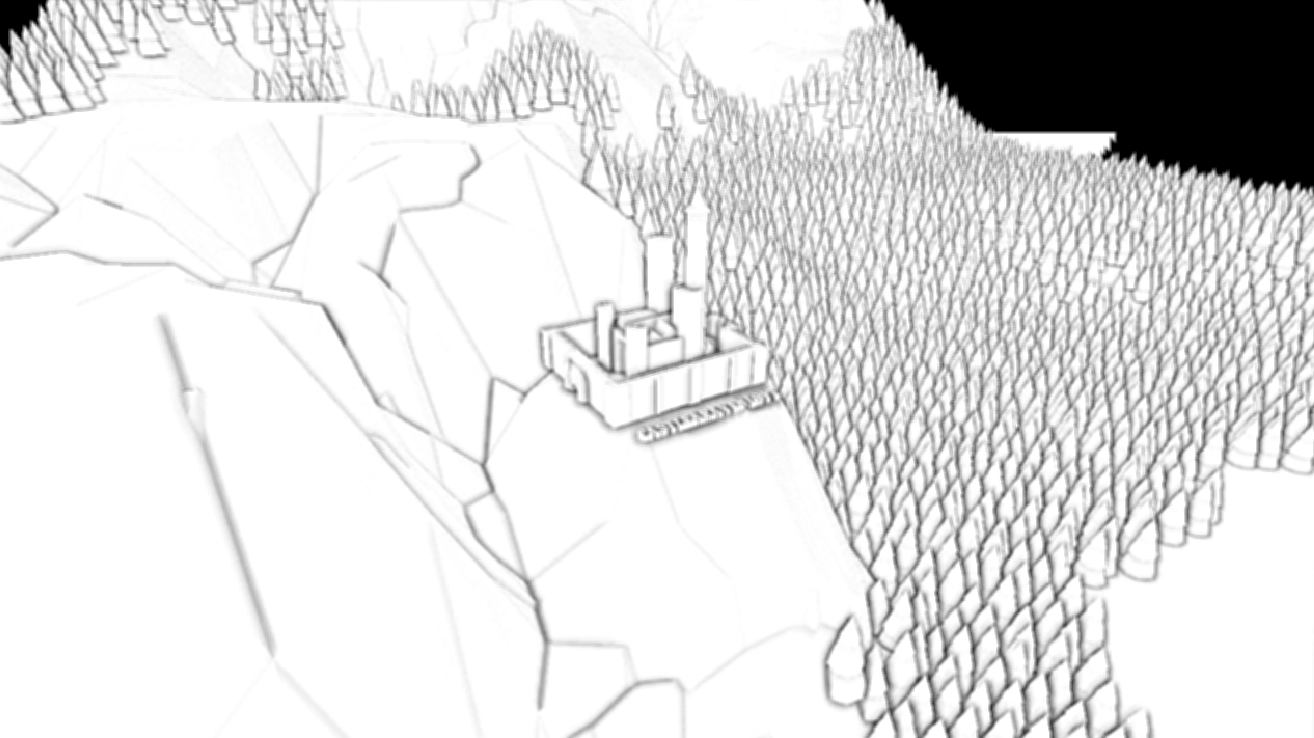
Ambient Occlusion after blurring
After this is the light shaft generation process. To my knowledge, this pass is non-standard and fairly specific for my particular use case, but it leverages some common techniques in volumetric rendering. The algorithm at this stage creates a ray from a given pixel's world space position to the camera's world space position value, then takes samples at certain points along the ray and tests whether they fall within the shadows from the shadowmapping pass. The amount of shading is then averaged across the sample positions within a zero to one range. Additionally, I have implemented tests to check whether a sample is inside a more specific volume (in this case a ground-based fog that hangs at a certain height). The same averaging is done for these samples and saved to another channel of the output texture. In theory, the output texture could support three light scattering volumes and a general atmosphere, but for this project I used only one extra volume for the fog. The described light shaft calculation algorithm is done entirely at a quarter of the final resolution, and the resulting texture is upscaled and blurred before being used in later steps to adjust the color of participating media.
Light shaft texture after upscaling and blurring
Main Render
After the prep stages are complete, the main render occurs and the final image starts to become visible. The textures are all sampled for each pixel on the screen. The final color is comprised of three major contributing factors: main lighting, atmospheric scattering, and fog.
The main lighting equation consists of three separate terms, the first is a representation of the amount of light received from the scene's light source, done using a simple dot product. Second is a hemispheric light, meant to represent ambient light coming in from all directions, this is a dot product against a vector straight up along the y-axis. Third is a cheap global illumination component, this simulates the light bounced off of nearby objects onto the faces that are hidden from direct light, this is done as a dot product against the negative of the light direction with the y-component zeroed out. Ambient occlusion is applied to the hemispheric and global illumination terms, but not the main light source component. This lighting model is based on an article by Inigo Quilez
Next, the amount and color of atmospheric scattering is calculated. The amount is 1 - the natural exponentiation of the distance times a fog constant (e.g. 1 - exp( d * b ) ) and color is a blend between the actual atmosphere's color, the main light source's color, and the value from the light shaft calculation step.
Then, the "ground fog" amount is calculated. This fog models a volume that occupies the space below a certain y - axis aligned plane with additional rippling on the surface to present a more organic shape. The color of the fog also has the value from the light shaft step applied.
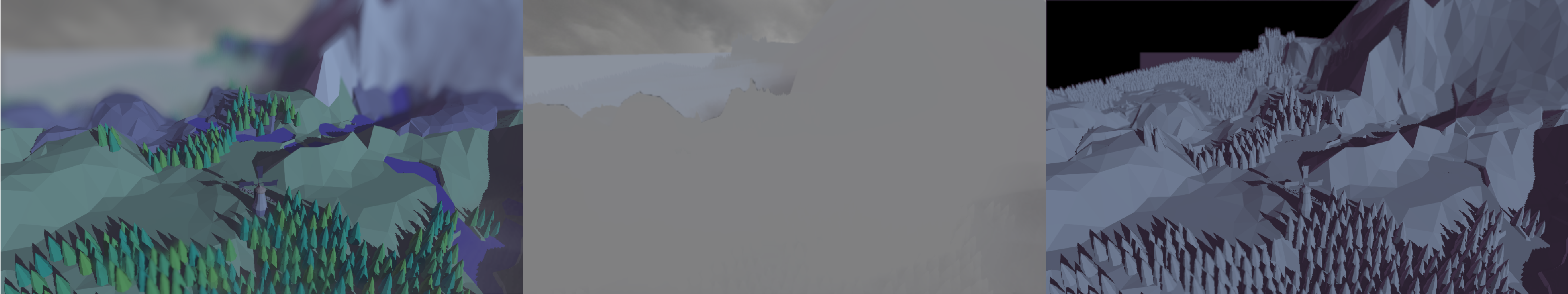
Light components: normal image, fog only, & light only
Once these three values have been calculated, they are combined into the final color, the first component serving as the base color and the two fog and atmosphere colors blended on top of that. This color is written out to three HDR render textures, with the alpha value dependent on the pixel's distance from the camera and whether it falls into a far field, near field, or mid field. Distinguishing between far/near/mid fields will be important in a future bokeh blur step.
Post Processes Stages
Finally, the last stage of the pipeline occurs. At this point the image has finished "rendering" and various post-effects are applied. The first such effect is anti-aliasing using the FXAA method. I won't re-describe the algorithm as it's well documented online, but I'll take a moment to justify it's use compared to other options. FXAA works well for "clean-edged" shapes with little to no high frequency detail in their surfaces. Essentially, I found it to be excellent for a "low-poly" look without any granular details. It also complements a deferred pipeline well where Multi-Sample anti-aliasing fails for technical reasons, and has a fairly low implementation cost when compared to a solution like Temporal Anti-aliasing. TAA offers better results for high-frequency details or organic, rough-edged shapes like hair and foliage, but I did not generally need such results for this project.
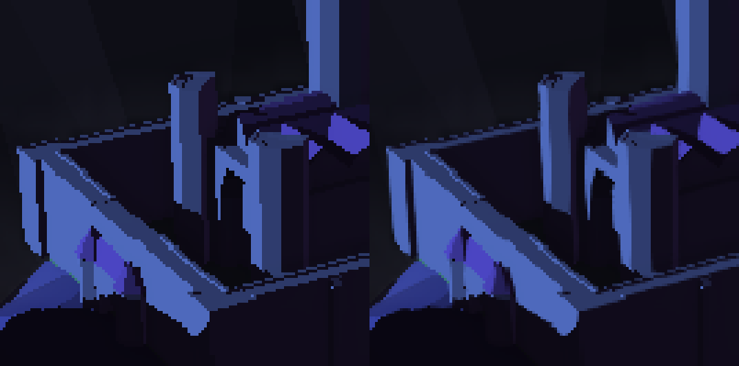
FXAA closeup, before & after
The second post-effect is the bokeh blur of the near and far field textures mentioned in the main render step. The blur is an unweighted average of samples from a set of points generated as a fibonacci-spiral with a catch - in the near field, samples that are from the mid or far fields are discarded without contributing to the final average. The radius of this spiraled sample pattern depends on the degree to which a given pixel is "in-focus." A small radius results in little blurring and vice versa. I stored the degree of blurring for each texture in the alpha channel with 0 being no blur (a 0 length radius) and 1 being a full blur. After blurring the far and near fields, the results are combined into one image with the anti-aliased texture from the FXAA step between the two. As a general note, there is another approach to such blurring that allows it to be done in a single pass, negating the need for separate textures and a combining step.
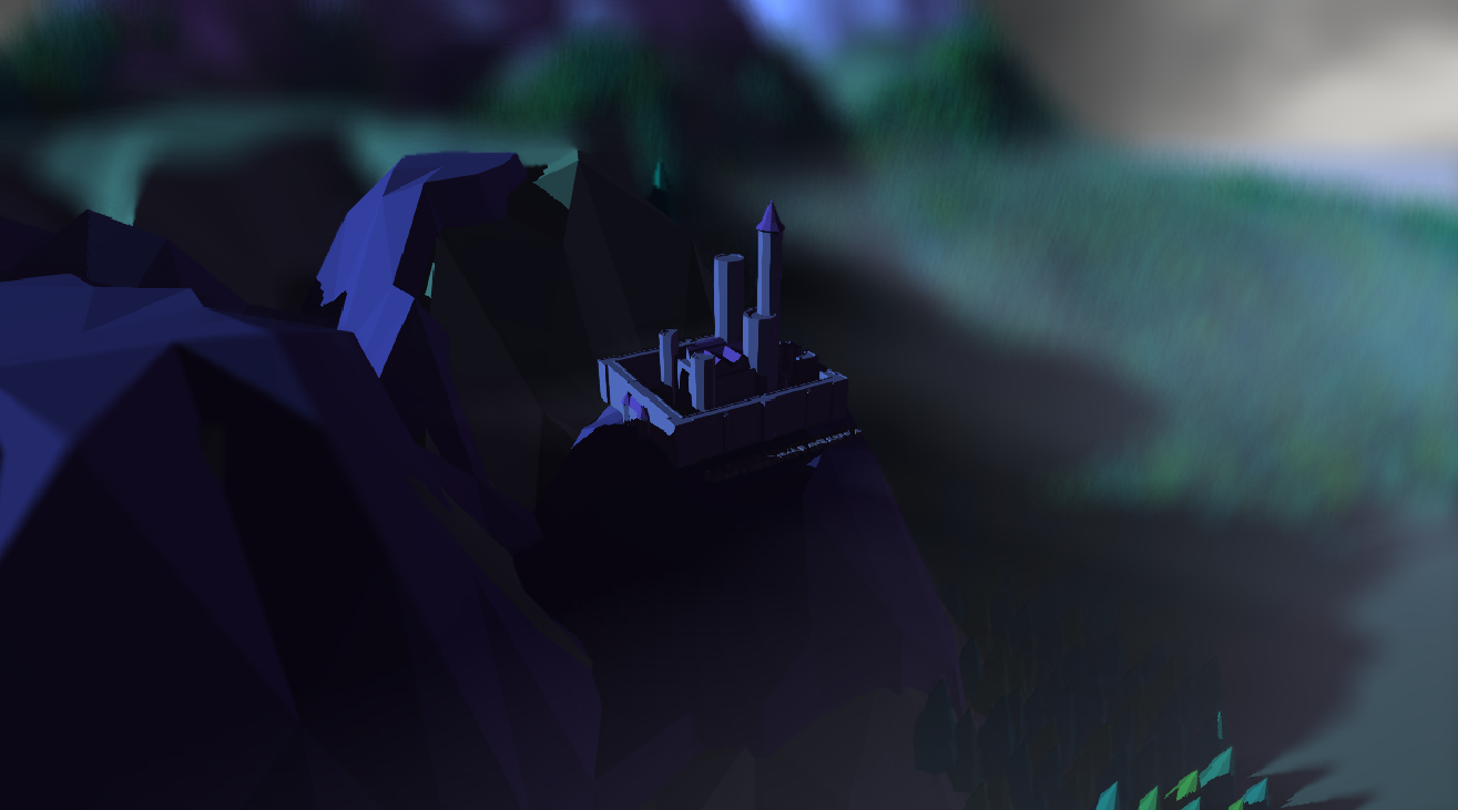
Render after Bokeh blurring
The final effect is mapping the HDR 16 bit floating point color texture to the actual display's LDR 8 bit unsigned integer buffer. There are many mapping functions out there, but I went with the "Uncharted 2 Tonemapper" due to its purported saturation of dark areas and potentially adjustable curve shape. Honestly, I don't really see good saturation in the darker areas of the image, but this could perhaps be caused by an inappropriate lighting setup or maybe I just don't have good taste.
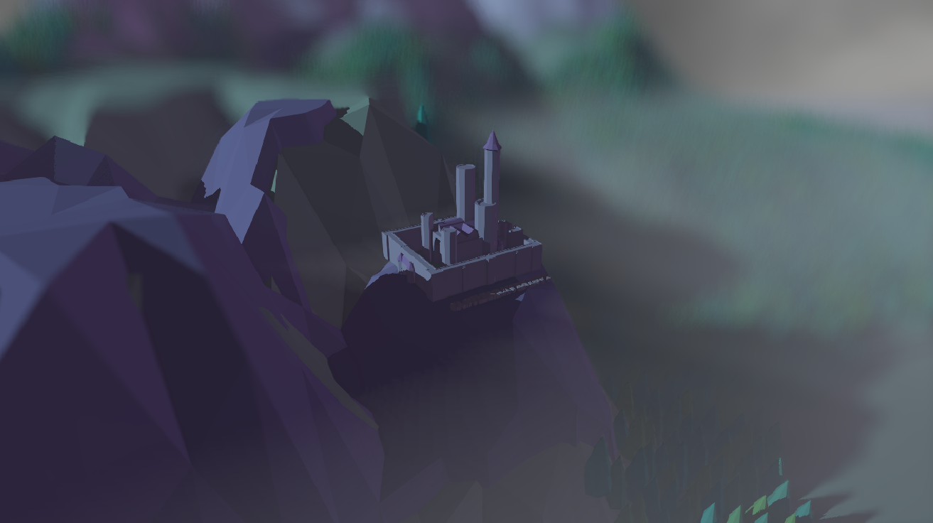
Final Tonemapped Image
With the tonemapping complete, we have reached the end of the pipeline and the final image is complete. This project represents about a year's worth of work, learning as I progressed. If you're in the middle of a similar project I hope this document can help with making choices in the your own work, and if you're learning I hope it can offer a jumping off point for learning these techniques in depth. Thanks so much for taking the time to read this.